Intro
Since a few years it is possible to learn playing Atari games directly from pixels with reinforcement learning1. A more recent discovery was that evolution strategies are competitive2 for training deep neural networks on those tasks. And even a simple genetic algorithm3 can work.
Those methods are fun to play around with. I have created a maze-world and trained a neural network to explore it. This task is much simpler than Atari but still gives interesting results.
I’m using Covariance-Matrix Adaptation (CMA-ES) and have tried a few simpler methods. The focus is on results but code is available.
Maze
This is my generated 2D maze8, featuring:
- Food (red)
- Agents (green)
- Traces (dark green)
The agents cannot die. They all use a copy of the same controller. The goal is to improve this controller so that the agents (together) find as much food as possible.
This video shows a mediocre controller in five random worlds:
Observations: The agents start moving in different directions, but later all drift in a random walk to the bottom right. Sometimes they eat food blobs. (They can actually move through walls with a very low probability9.)
Agent Controller
The controller is a neural network with fixed topology10 and learned weights. The architecture is pretty standard except for the memory11.

Inputs:
- The agents are nearly blind. They only see walls and food next to them.
- The agents don’t know their previous action. To keep going into a new direction they must learn how to use the external memory.
- The trace count can detect crowded areas. It includes the agent’s own trace.12
Outputs:
- The softmax makes it simple to output fixed probabilities over actions, like “60% down, 40% left”.
- An output with high certainty (“99.9% down”) requires larger weights, which can only appear later during training.
The network has a single hidden layer and about 1‘000 parameters (weights and biases).
The parameters are optimized directly. The setup violates some assumptions13 for standard (value-based) reinforcement learning, but a direct search for the parameters does not rely on those assumptions.
Training
Inspired by the Visual Guide to Evolution Strategies5 and by remarks in various papers I have used the Covariance-Matrix Adaptation Evolution Strategy (CMA-ES). It worked with practically no tuning. I have tried other black-box optimization methods (discussed below) but was unable to reach the same score.
I dare to compare CMA-ES with the Random Forest Classifier6: a strong baseline that works out-of-the-box and is difficult to beat. Though it only works up to a few thousand parameters.
Here is a summary: CMA-ES tracks a Gaussian distribution (with full covariance) over the parameters. The user provides an initial estimate of the scale of each parameter (variance). CMA-ES will then sample a small population, evaluate it and sort by fitness. This rank information is used to update the distribution, and the process repeats.
For a better overview, see “What is an Evolution Strategy?” from the same guide. The general principle is easy to understand, but the details are a bit involved. With CMA-ES you really should be using a library (pycma) and not implement from scratch.
Training plot:
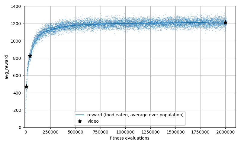
Each generation is evaluated on a different set of random maps. There is a lot of fitness noise because of this. The moving average shows a slight upwards trend at the end.
It takes about an hour to reach an average score of 1‘000 on my low-end PC. It takes about ten hours on an AWS c5.9xlarge instance to reach the score above14.
After 44‘000 evaluations (second video):
Observations: The agents now keep changing directions. Sometimes they jitter around for a moment, especially when they should be turning. They can escape from dead ends, but it requires many attempts if the exit is narrow.
And finally, after 2‘000‘000 evaluations:
Observations: The winning strategy follows the left wall at a short distance. In empty space it prefers straight lines with random left-turns. At the end of a horizontal line of food the agent usually turns 180 degrees and finds back to the remaining food blob.15
Discussion
CMA-ES is known to work well with tens to hundreds of parameters. With just 1‘000 parameters we are already approaching its limits. This may be a bit disappointing, because the learned strategy does not look really complex. I expect that the model could be improved to fit the task better, reducing the number of parameters.
To put the network size into context: six parameters are enough to learn the classic cart-pole balancing task; 5‘000 have been used to control a simple 2D-Hopper robot; and 33‘000 to play Atari games from pixels4, though four million have also been used3.
Other evolution strategies can scale up. But CMA-ES can achieve amazing results with smart use of a few hundred parameters, like this Muscle-Based Locomotion for Bipedal Creatures7.
I have tried a few simpler methods. A simple GA (not shown here), the Cross-Entropy Method (CEM) and differential evolution. They all got stuck in local optima.
Here is an impression of my attempts to find good CEM parameters:
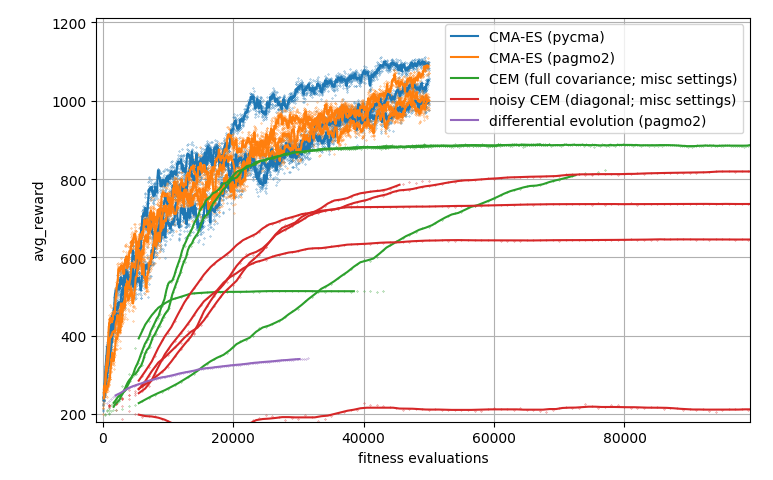
(The CMA-ES lines have more noise because they use a smaller population size of 23 per generation, while other methods use between 200 and 1000. The dots show the fitness per generation before filtering.)
This is a different (older) variant of the task which is faster to train. As you can see, it is not a trivial optimization problem.
One big challenge is the evaluation noise caused by the random maze generator. One lucky maze can have lots of food exactly where the agents are going. Some algorithms will give this score too much credibility, and use that lucky controller as a starting point for most mutations. Until the score gets beaten by an even more lucky evaluation. I think this is why differential evolution failed here.
I have also tried variations of the neural network:
-
The controller did surprisingly well when I removed the hidden layer. It finds good solutions much faster. Maybe the memory feedback loop helps with that. But the advantage of using a hidden layer becomes clear after 3‘000 evaluations.
-
The performance difference between 20 and 40 hidden neurons is not that large. With 20 neurons it trains faster (only 600 parameters). The defaults of CMA-ES worked great with 20 hidden nodes, but I have found that increasing the population size from 23 (default) to 200 helps with the larger network.
-
A good scaling of the initial weights can speed up the first learning phase a lot. The same is true for input and output normalization. But this advantage often shrinks down to zero long before the final score is reached. Initialization should become more important with additional hidden layers. It’s known to be critical for deep neural networks.
Code
Code is available in my pixelcrawl GitHub repository. It is not very polished, however it is reasonably optimized (at the expense of flexibility).
The original version was pure Python. It was about 100x slower than the current Python/C++ mix. There is a lot access to individual pixels and math involving small arrays, something which Python is really slow at.
Bonus
Can it survive in empty space? Or will it always stick to the walls?
Let’s transfer the trained agent into a new environment:
Observations: The learned strategy is somewhat robust and looks well randomized. It has trouble getting into certain one-pixel cavities. But it keeps exploring.
-
Playing Atari with Deep Reinforcement Learning, Mnih et al., 2013. ↩
-
Evolution Strategies as a Scalable Alternative to Reinforcement Learning, OpenAI blog, 2017. With accompanying paper Salimans et al., 2017. ↩
-
Deep Neuroevolution: Genetic Algorithms Are a Competitive…, Such et al., 2017. With related article Welcoming the Era of Deep Neuroevolution, Uber blog, 2017. ↩↩
-
Trust Region Policy Optimization, Schulman et al., 2015. ↩
-
A Visual Guide to Evolution Strategies, blog post by David Ha (hardmaru), 2017. ↩
-
The Unreasonable Effectiveness Of Random Forest, blog post by Ahmed El Deeb, 2015. ↩
-
Muscle-Based Locomotion for Bipedal Creatures, Geijtenbeek et al., 2013. Video and paper. ↩
-
How do you generate a maze? Simple.
Perlin Noise and a threshold.Start from a noise image and apply a 3x3 binary filter repeatedly. There are 2512 possible filters to choose from. Most of them transform noise into noise. Pick one that produces a low number of horizontal and vertical edges. Using this as a fitness measure, the Cross-Entropy method can find a good filter. If you’re not happy with the result, use novelty search to evolve filters with maximum diversity. To measure the diversity of 2D patterns, use the first few layers of a pre-trained ResNet50 to extract basic visual features. This should result in different textures. Pick one that looks like a maze. Simple as that. ↩ -
In early experiments I used a higher probability to move through walls because it was possible to start inside of a wall. The agents liked this a bit too much, especially when I gave them more time to explore. Drifting through walls in a fixed direction is a sure strategy to explore the whole maze, including disconnected parts. Whenever they got stuck they moved into the next wall instead of searching a way around. ↩
-
A well-known alternative would be to evolve the topology together with the weights using NEAT. I have not tried this, but it’s known to work well for small networks. During the deep learning hype this approach was not getting much attention. Now the evolution of topology seems to be coming back as architecture search for deep vision networks. There is also recent work happening on indirect encoding (e.g. evolving regular patterns). See Designing neural networks through neuroevolution (Stanley et al., 2019) for a recent overview. ↩
-
Using
memory[t+1] = 0.99 * memory[t] + 0.01 * outputs[t], so the memory is just a low-pass filtered version of the outputs. A standard recurrent neuron could have learnt this rule. The memory half-time of about 70 steps (1/-log2(0.99)) was found to work well. I have also attempted to learn individual half-times for all 6 memory cells, so far without success. I have not tested other structures, but it seems to be working okay. At first I initialized the memory (the filter states) with zeros. But a swarm of 200 agents performed much better with random initialization, because it gives each agent access to a different (somewhat constant) input. This helps to spread out early. ↩ -
The trace input is a left-over from early experiments with 200 agents swarming the maze. It was meant to detect and avoid crowded areas. But 200 agents were very confusing to watch and the strategy mostly resembled a flood-fill algorithm. I’m not sure if or how the current agents use this input. ↩
-
Standard RL methods like Q-learning expect to be solving a Markov Decision Process (MDP) that is fully observable. However the nearest four pixels are lacking a lot of information about the state. A memory is evolved to extract relevant information from the past. For the evolution strategy this is just some additional parameters to optimize, and never mind the feedback loop this creates. When learning Atari games the inputs are usually extended to include some history, e.g. the last four video frames, in the hope that all relevant state information can be extracted. A different issue is that the network controls only a single agent. It would be straight-forward to maximize the reward of this agent with standard RL. But it is not clear how prevent competition and maximize the collective reward of all agents instead. ↩
-
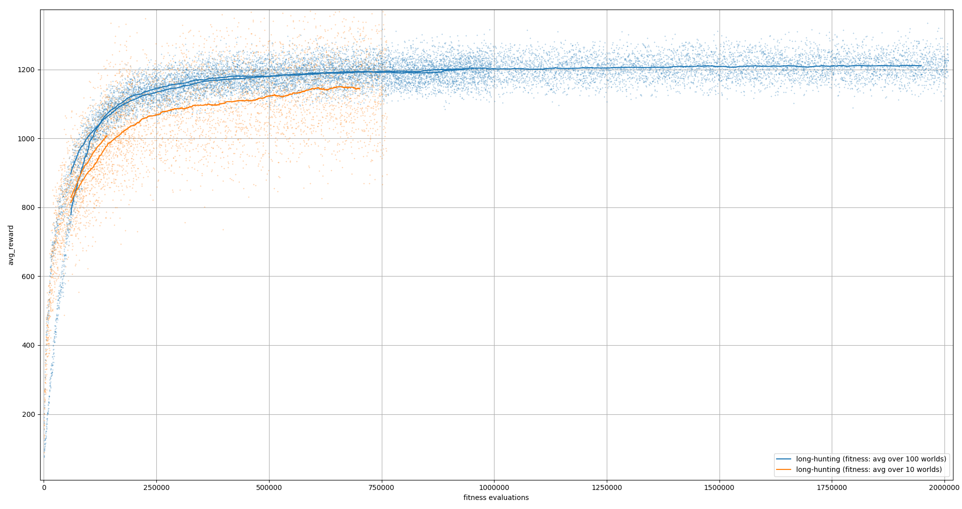
The run presented here actually took a few days, because I was evaluating each agent on 100 maps instead of 10. This was complete overkill. It helps, but not enough to justify 10x training time. Training was done on AWS spot instances because they are cheap. They can be interrupted at any time, and I’m just counting on my luck; so far I’ve seen only two interruptions. Previously I used dask distributed with a central scheduler and spot instances as workers for a different experiment. This was quite involved to manage. For now I’m back to plain dask to use multiple cores and good old rsync and ssh.
There is also a scaling issue that I didn’t get around to debug yet: the 36 vCPUs of the c5.9xlarge instance are utilized only at 40%. (Update: it’s mostly caused by the non-parallel CMA-ES update step, which must wait for all parallel evaluations to complete before starting new ones.) There is no point going distributed if the largest AWS instance (72 vCPUs) cannot be saturated. The price per vCPU is nearly the same for small and large instances. ↩ -
Remember that the agent cannot see when a food blob has ended, only that all four directions are empty. It must therefore be using its memory to prepare the correct turn-around. Also, the agents sometimes leave crumbs of food that they should have noticed. Probably a fast exploration of the maze has higher priority than collecting every bit of food. It’s also likely that it lacks the memory capacity to remember long enough. The videos actually run twice as long as an episode. The fitness is the amount of food collected in the first half of each video-episode. At this point there are usually big blobs left, which are more important than the crumbs. ↩